
The Problem
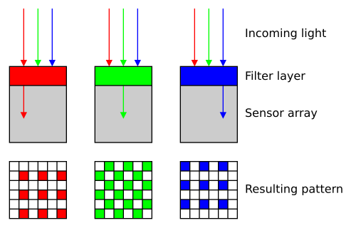
Digital camera sensors can only capture one colour per pixel through a colour filter array, creating a mosaic pattern called a Bayer Pattern. The full-colour images we see require sophisticated algorithms to reconstruct the missing colour information at each pixel location. This process is called demosaicing.
The Solution
This project implements a machine learning-based demosaicing algorithm using linear regression to predict missing colour values. By training on over 300,000 image patches from diverse scenes, the algorithm learns optimal coefficient matrices that leverage the correlation between neighbouring pixels and colour channels to reconstruct full-colour images.
Results Overview
The linear regression model consistently outperformed MATLAB’s built-in demosaic function across all test images, achieving lower Root Mean Squared Error (RMSE) values and producing fewer visual artifacts.
My Linear Regression Model
4.99
Average RMSE
MATLAB's Built-in Function
6.05
Average RMSE
Key Performance Metrics:
- Staircase Image: 6.07 vs 7.75 RMSE (28% improvement)
- Seaside Houses: 7.78 vs 9.16 RMSE (18% improvement)
- Swing Set: 1.11 vs 1.25 RMSE (13% improvement)
Skills Applied
Background
The Bayer Pattern
Modern digital cameras use a Colour Filter Array (CFA) where each pixel sensor is covered by a red, green, or blue filter. The most common arrangement is the Bayer pattern, which has twice as many green pixels as red or blue to match human visual sensitivity. This creates four distinct mosaic patterns depending on pixel position.
Bayer Colour Filter Array showing the RGGB pattern where each pixel captures only one colour channel.
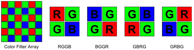
Four distinct 5×5 mosaic patterns made from the CFA.
Why Linear Regression?
Natural images exhibit strong spatial correlation since neighbouring pixels tend to have similar values (brightness in surrounding pixels indicates brightness in a missing pixel). Additionally, colour channels are correlated with each other (high levels of red in surrounding pixels indicates higher levels of red in a missing pixel). These properties make it possible to approximate missing colour values as linear combinations of surrounding known pixels.
For a 5×5 patch of pixels, the missing colour component at the center can be predicted as:
Where:
is the missing green component at the center pixel
is the coefficient matrix learned from training data
is the 5×5 mosaic patch of surrounding pixels
and
are individual elements of the matrices
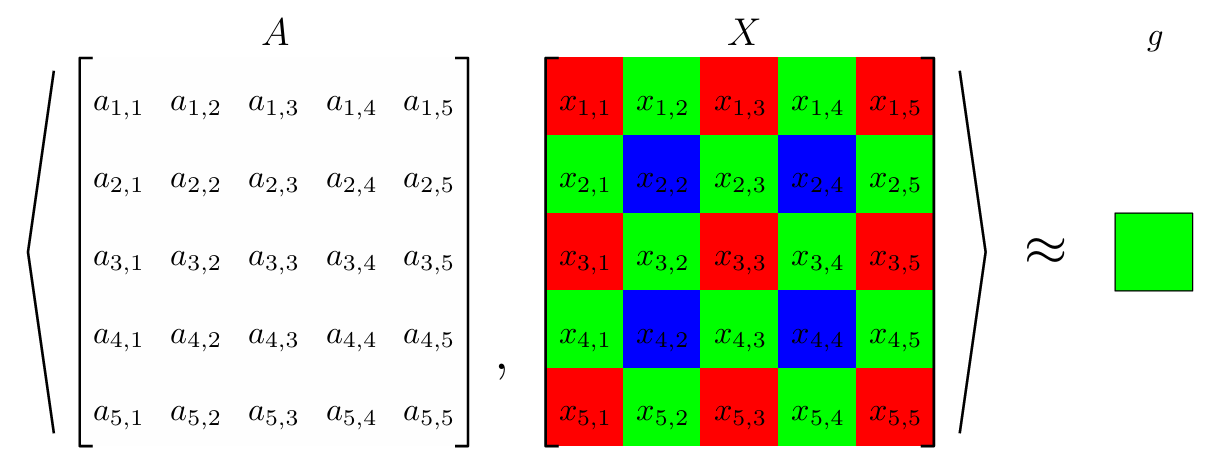
Estimating missing green component.
The optimal coefficient matrix A is found by training on thousands of image patches where both the mosaic pattern and ground truth colours are known, minimizing the squared difference between predicted and actual colour values using least squares regression.
Implementation Details
Bayer patterned image
Reconstructed image
Training Process
1. Data Collection
- 5 diverse training images (300,000 total patches)
- Random 5×5 samples from each Bayer pattern configuration
- Ground truth values extracted from original full-colour images
2. Coefficient Calculation
Each pixel position has a unique neighbourhood pattern of known colours surrounding it due to the Bayer filter arrangement. Since each position needs to predict 2 missing colours, we require 4 positions × 2 colours = 8 coefficient matrices total.
For each configuration, the optimal coefficients are found by solving a linear least squares problem. Given n training samples (mosaic patches ) and their corresponding ground truth colour values (
), we find the coefficient matrix A that minimizes the total prediction error:
This optimization problem can be solved analytically using the linear least squares method. After reshaping each 5×5 patch into a 25-element vector and stacking all training samples into matrix X, the optimal coefficients are computed as:
Where X is the matrix of all training patches (each row is one flattened 5×5 patch), g is the vector of ground truth values, and b contains the learned coefficients. This process is repeated eight times to create specialized coefficient matrices for each Bayer pattern configuration and colour prediction.
3. Reconstruction
For each pixel in a test image:
- Extract surrounding 5×5 neighbourhood
- Identify Bayer pattern configuration at that location
- Apply appropriate coefficient matrices
- Predict missing colour values
- Combine with known value to create full RGB pixel
Visual Comparison
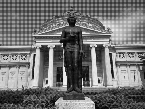
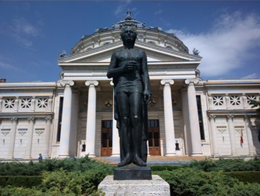
Staircase Test Image
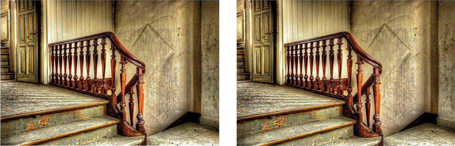
Staircase test image comparing MATLAB's demosaic function (left) with regression model (right).
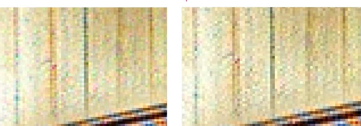
Zoomed in staircase test image comparing MATLAB's demosaic function (left) with regression model (right).
The staircase image presented significant challenges with sharp colour transitions and limited colour variety. The regression model better preserved true colours of vertical wall stripes and reduced striping artifacts along the banister (bottom right).
Seaside Houses Test Image

Seaside houses test image comparing MATLAB's demosaic function (left) with regression model (right).
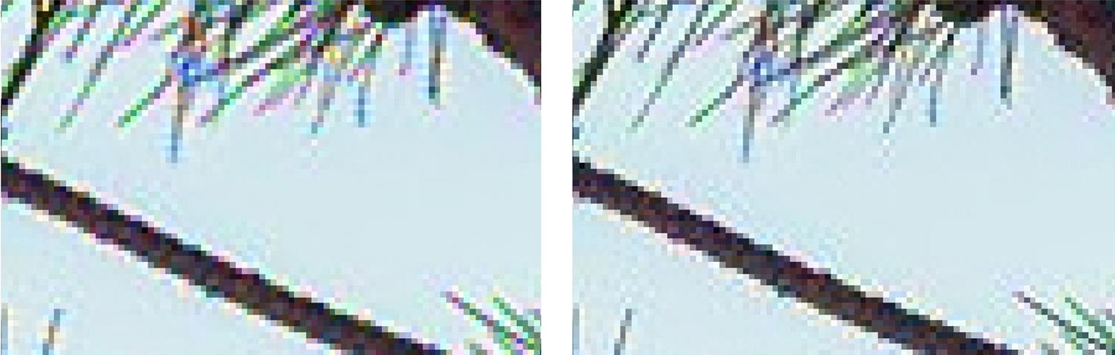
Zoomed in seaside houses test image comparing MATLAB's demosaic function (left) with regression model (right).
High-contrast scenes with bright colours and sharp transitions revealed clear differences. Tree branches in the zoomed view showed more consistent brown colouring with fewer zipper artifacts in the regression model.
Swing Set Test Image
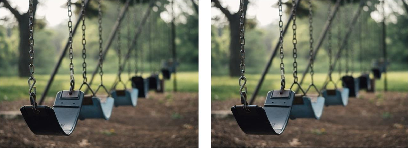
Swing set test image comparing MATLAB's demosaic function (left) with regression model (right).
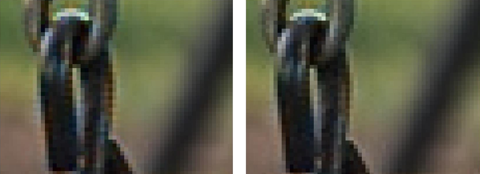
Zoomed in swing set test image comparing MATLAB's demosaic function (left) with regression model (right).
The blurred background created smoother transitions, allowing both algorithms to perform well. However, the regression model still showed reduced artifacts on the swing chain in foreground details.
Training Images


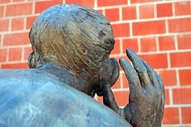
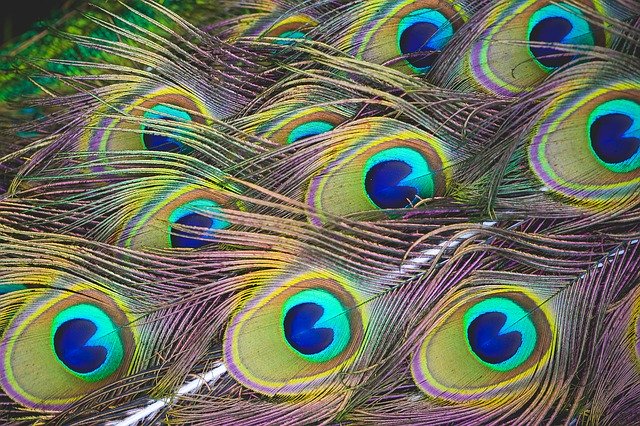

Five diverse training images used to generate 300,000 random 5×5 patch samples for coefficient learning.
Grade: 110/100 (Bonus awarded for outperforming MATLAB’s algorithm)
| Course: COMPENG 3SK3: Computer-Aided Engineering | McMaster University | January 2023 - April 2023 |